For years, companies tracked their environmental impact mainly through carbon emissions. Carbon is interchangeable: absorbing a ton of CO2 in one country cancels out a ton released anywhere else in the world.
Biodiversity — the variety of plants, animals, and natural habitats—does not work that way. Nature is strictly tied to specific places. Protecting a wetland in Europe cannot make up for destroying a rainforest in South America.
Because local ecosystems cannot be swapped or offset elsewhere, harming a specific habitat exposes companies to direct problems: supply chain disruptions, legal penalties, and lasting reputational damage.
Measuring nature, however, is much harder than tracking carbon. Without clear boundaries and reliable measurements, companies often rely on basic headcounts of local animals and plants. But simply counting species can hide deeper environmental damage. This leaves businesses open to accusations of greenwashing and puts them at risk of failing to meet official reporting rules.
In this article, you will learn:
✅ How to look at biodiversity locally and regionally—distinguishing between what is on a single site, how much nature changes between your different sites, and the total biodiversity across the entire region
✅ Why only counting how many species exist is misleading and how to distinguish between species richness and species evenness
✅ How Hill numbers convert abstract scores into intuitive numbers that business executives, auditors, and sustainability teams can interpret
✅Why knowing the overall health of the wider region is essential for setting realistic sustainability targets and meeting disclosure requirements
✅How to identify which of your company's facilities operate in rare, irreplaceable ecosystems versus common ones, helping you prioritize where environmental damage poses the highest operational and regulatory risk
By the end of this article, you will understand the foundational concepts and mathematical framework needed to structure and interpret biodiversity measurements across your operations.
2. Measuring biodiversity across alpha, beta, and gamma scales
Before a company starts running field studies, setting environmental goals, or asking suppliers for biodiversity data, it must first draw clear boundaries around the specific areas it impacts.
Unlike climate metrics, biodiversity cannot be evaluated as a single, global metric. Ecological health changes dramatically depending on whether you zoom in on a 1-meter field plot, an entire industrial facility, a shared river basin, or an international supply chain.
Without defining spatial scale, questions like “How biodiverse is our supply chain?” lead to misleading conclusions:
On a single farm: A supplier’s land might look healthy and full of life because it is filled with common, adaptable wildlife, like standard weeds, insects, and birds that can survive anywhere.
Across the whole region: If hundreds of those identical farms replace native forests, wetlands, and grasslands, the entire landscape becomes one monoculture. The wider region loses its rare, specialized species and the natural wildlife pathways connecting them.
Evaluating sites in isolation hides regional damage, leading to flawed risk assessments and misdirected sustainability investments.
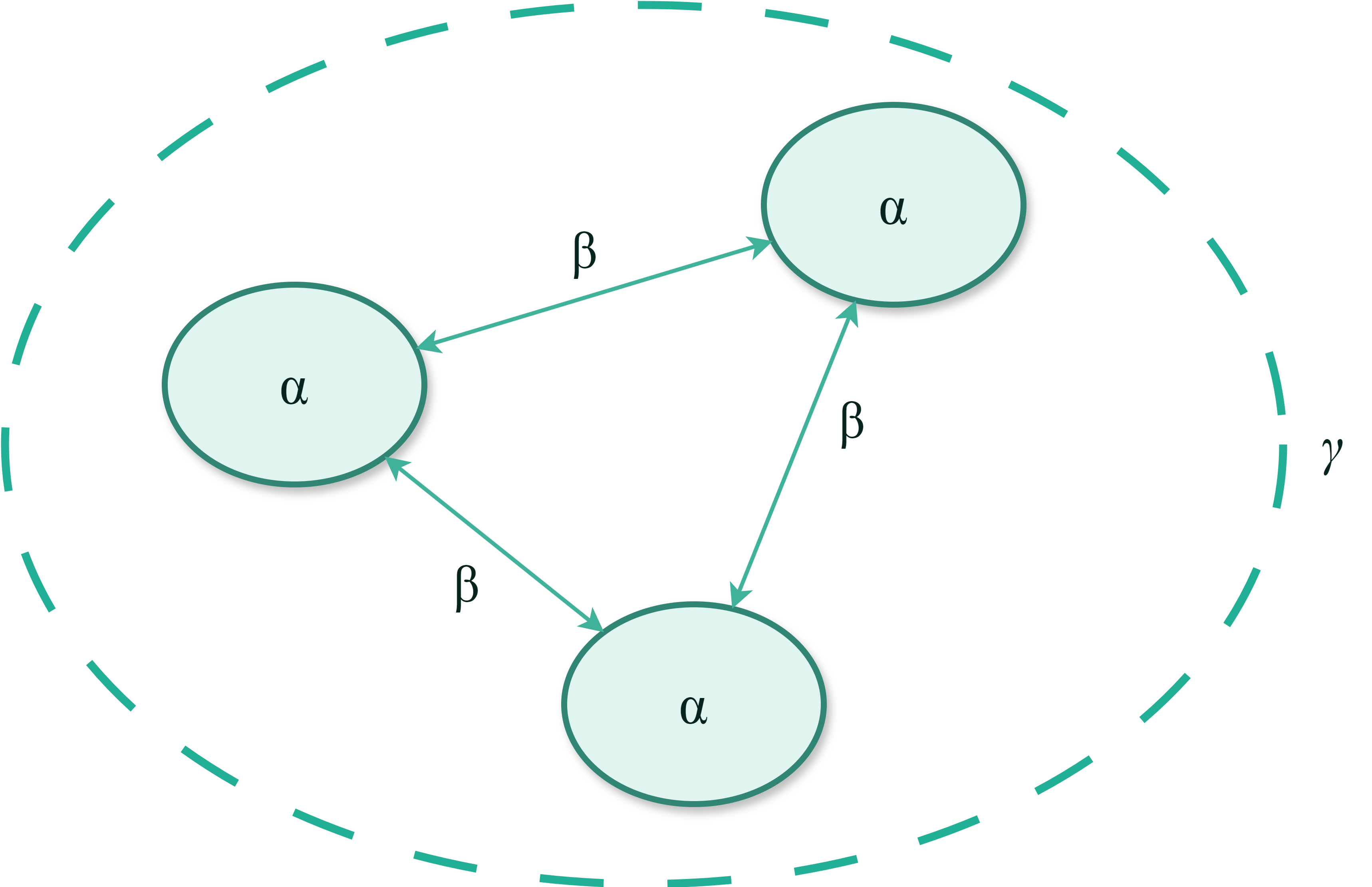
To solve this, organizations use spatial partitioning—measuring biodiversity across three distinct scales: alpha, beta, and gamma diversity.
Alpha diversity (α)
Measures the variety and balance of species living within a single location (such as one farm, factory, or facility). It is the main metric for tracking your direct footprint on that plot of land over time and seeing if local conservation efforts are working.
Beta diversity (β)
Measures how much the wildlife changes from one site to another. So, it answers the question howSite A differs from Site B. If all your locations have identical wildlife, beta diversity is low. If each location hosts unique species, beta diversity is high.
Gamma diversity (γ)
Measures the total biodiversity across a whole region (such as an entire river basin, forest system, or territory). It gives you the big-picture view, helping you determine whether the combined footprint of all operations in the region is supporting or degrading the regional ecosystem.
Example Imagine a renewable energy company operating wind farms across a mountain range:
Alpha diversity
Counting wildlife at one specific facility, for example, finding 15 bird species at Wind Farm A.
Proves local environmental compliance and secures building permits for that specific plot of land.
Beta diversity
Comparing species between locations. Wind Farm A (coastal) and Wind Farm B (inland) might both have 15 bird species, but zero species in common—meaning 30 completely different species across both sites.
Prevents a one-size-fits-all mistake. If the wildlife at each location is entirely different, using identical environmental protection plans for both sites will fail to protect local wildlife.
Gamma diversity
The total variety of wildlife across the entire mountain range (15 species at Site A + 15 at Site B + 10 in the connecting natural corridors = 40 total bird species).
Delivers the big-picture view. It shows whether the combined footprint of all activities in the region is protecting or degrading the regional ecosystem.
Importantly, this framework is not limited to counting species at a physical site. It scales across all three foundational tiers of biodiversity: Genetic, Species, and Ecosystem diversity (read more in the previous article: Understanding biodiversity).
Because spatial partitioning is a flexible mathematical tool, alpha, beta, and gamma apply no matter which biological tier you are assessing:
Genetic tier
Alpha: The variety of genetic traits within a single local group. It shows how adaptable that specific local population is to immediate stressors.
Beta: The genetic differences between separated groups. It reveals whether distinct populations carry unique traits that help them survive localized diseases or environmental shifts.
Gamma: The total gene pool across the entire region. It measures the overall genetic health and long-term evolutionary resilience of the species as a whole.
Species tier
Alpha: The number and balance of species living on a single property or operational site.
Beta: The species turnover between locations, measuring how many new, unique species there are as you move from one site to another.
Gamma: The total count of unique species thriving across the entire regional landscape.
Ecosystem tier
Alpha: The variety of habitats contained inside a single site boundary (such as a mix of wetlands, meadows, and tree canopy on one site).
Beta: The variation in habitat types across the region, showing how different the environments are from one site to the next.
Gamma: The complete picture of all interconnected ecosystem types across the entire regional biome.
3. How to measure biodiversity
To measure biodiversity accurately across individual sites, site-to-site differences, and entire regions, companies combine modern on-the-ground monitoring tools with ecological math.
Step 1: Collect ecological data
Before calculating biodiversity scores, companies gather raw data on what lives within and around their operations using four main monitoring methods:
On-the-ground field surveys: Ecologists physically inspect sample plots and walk set paths to identify species and count individual plant and animal populations firsthand.
Environmental DNA (eDNA): Teams collect water, soil, or air samples to test for microscopic genetic material (skin, hair, or waste) left behind by animals. This reveals which species use the area without having to physically catch or see them.
Bioacoustics: Automated sound recorders are placed across the land to continuously capture wildlife sounds, such as bird, bat, and frog calls, which specialized software then analyzes to identify active species.
Satellites and remote sensing: High-resolution satellite imagery and aerial laser mapping (LiDAR) track the big picture, measuring overall plant health, tree canopy structure, and habitat connectivity across the wider region.
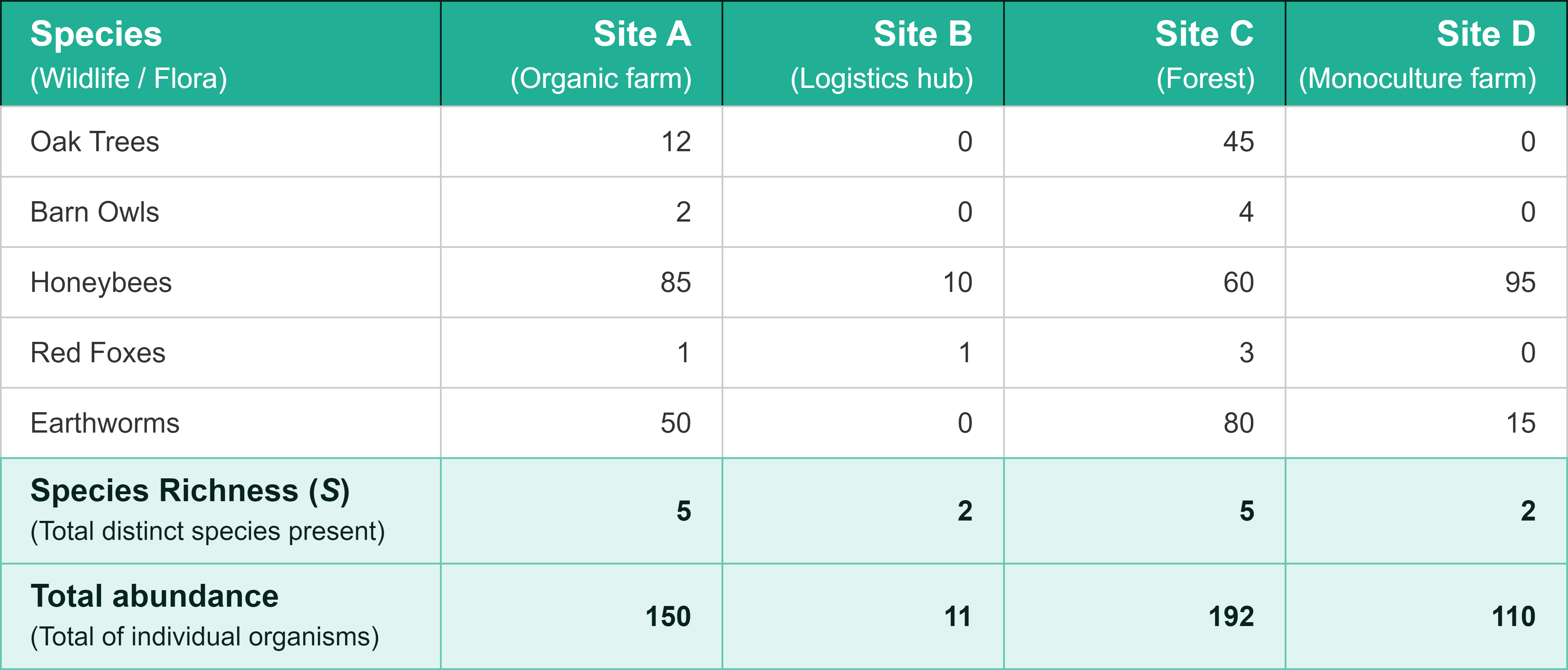
The raw field data is structured into a site-by-species matrix (recording species presence and counts per site):
This field data supplies the inputs needed for your three diversity scales:
Data for alpha diversity: You need the species list and population counts from each facility or plot. This measures local site health and tracks your direct operational footprint over time.
Data for gamma diversity: You combine the species found across all your company’s sites with public data from the surrounding natural landscape (such as neighboring forests, rivers, and protected areas). You can pull this regional data from open platforms like GBIF (Global Biodiversity Information Facility), national wildlife registries, or local university studies. This measures the total regional species pool.
Calculating beta diversity: You do not measure beta diversity directly in the field. Instead, you calculate it mathematically by comparing your local site data (alpha) against the regional total (gamma) or across your different sites. This reveals how unique each location is and whether certain properties host rare species.
Step 2: Calculate local site diversity
Alpha diversity measures local diversity within a single operational site or facility footprint.
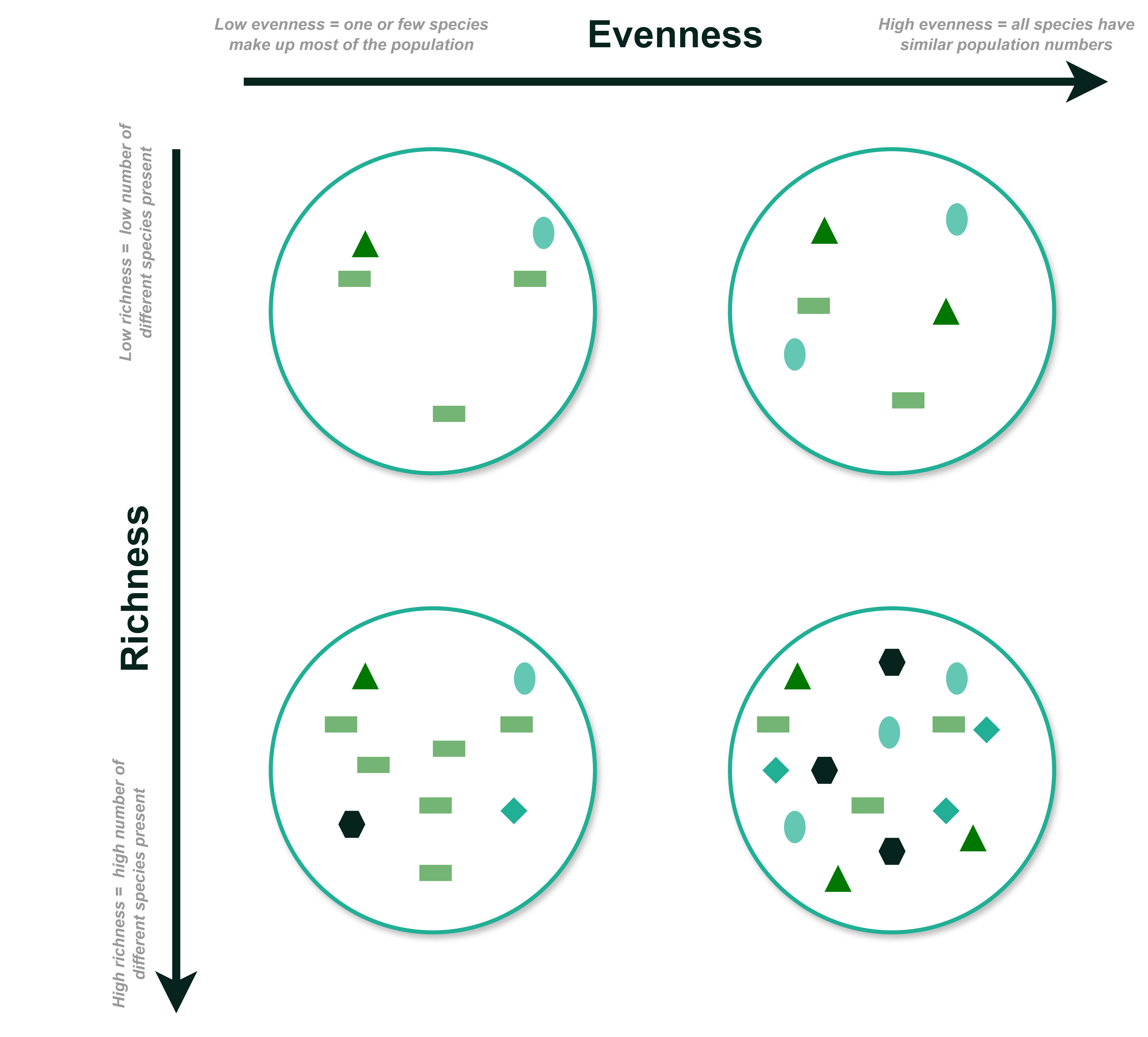
Before calculating this, it is important to know the distinction between species richness and species evenness:
Species Richness (S): The absolute count of distinct species present within a defined boundary.
Species Evenness: How balanced the population numbers are among those species. Is one species dominating the space, or is the population evenly spread?
Relying solely on species counts (S) creates dangerous blind spots in corporate risk management and natural capital accounting.
Example Imagine a corporate campus with 100 birds representing 10 different species. If 91 of those birds are common pigeons and only 9 belong to the other 9 rare species, the site technically has high species richness (S = 10), but extremely poor species evenness, meaning the ecosystem is heavily skewed and fragile.
Conversely, a site with 10 birds evenly split across those same 10 species has high evenness and far greater ecological stability. Relying on simple species counts (S) in ESG reports masks this imbalance, leading companies to claim high local alpha diversity on paper while unknowingly managing a degraded, highly vulnerable site.
Shannon Diversity Index (H’)
So how then to measure? While species richness (S) is simply: The total count of distinct species found at the site (n). One can also use the Shannon Diversity Index H’.
\(H' = -\sum_{i=1}^{S} p_i \ln(p_i)\)
I will not be explaining the mathematical formula here, but what it does is combine both species count (richness) and numerical balance (evenness) into a single score. It penalizes sites dominated by a single species and rewards sites where populations are evenly distributed. A higher H' score indicates a well-balanced, resilient site ecosystem.
Simpson Diversity Index (D)
This index measures the probability that two randomly picked organisms belong to the same species. It heavily focuses on dominant species.
\(\text{Simpson's } D = \sum_{i=1}^{S} p_i^2\)
Without getting into the math, this metric focuses on ecosystem dominance.
By calculating the probability that two randomly chosen organisms belong to the same species, it filters out rare sightings and highlights how many dominant species control the site.
Because the original Simpson’s Index measures sameness (meaning a higher score actually means lower diversity), ecologists usually convert it into one of two practical metrics:
Gini-Simpson Index (1−D): Measures the chance that two randomly picked organisms belong to different species, scored on a scale from 0 to 1:
A score of 0 means a complete monoculture (every single organism belongs to the same species).
A score of 1 means maximum possible diversity (every single organism you encounter is a completely different species).
Inverse Simpson Index (1/D): Converts the probability into an intuitive headcount of dominant species.
Instead of an abstract decimal, it gives you a number. For example, a score of 4 means the habitat behaves as if it is evenly shared by 4 major, dominant species, filtering out rare, one-off sightings that might skew the data.
Where Shannon (H’) gives you a complete picture of overall site balance, Simpson (D) acts as a stress test, revealing whether your site is diverse or overrun by one or more dominant species.
Example
Imagine two corporate sites, each home to 1,000 total animals across 10 different species:
Balanced forest: Each of the 10 species has 100 individuals (10% each). The populations are evenly balanced, creating a healthy, resilient habitat.
Degraded plot: 910 of the animals belong to one single dominant species (91%), while the remaining 9 species have only 10 individuals each (1% each).
Standardizing diversity with Hill Numbers (ⁿD)
Traditional ecological indices, such as the Shannon Index and Simpson Index generate abstract scores that create major communication barriers in executive reporting and ESG disclosures:
Non-linear scales: Diversity indices are mathematically non-linear. If a site’s Shannon score improves from 2.0 to 4.0, biodiversity has not simply doubled. In functional terms, it has increased by more than sevenfold.
Lack of practical meaning: Telling an auditor or board member that a facility scored 0.85 on Simpson’s Index or 2.71 on Shannon’s Index offers no tangible insight into whether the site is ecologically healthy, resilient, or degraded.
No common unit of measurement: Because different indices use entirely different units (or unitless scales), environmental teams cannot easily compare site-level gains against regional baselines.
To bridge the gap between complex ecological mathematics and corporate disclosures, ecologists convert these abstract scores into a unified metric called the effective number of species, formally known as Hill Numbers.
Instead of outputting an abstract decimal, the effective number of species calculates an equivalent benchmark:
“If every species in this habitat had perfectly equal population numbers, how many species would be required to produce this same level of ecological diversity?”
In nature, populations are rarely equal. A site with 50 recorded species where a single species accounts for 99% of all organisms does not function like a healthy 50-species ecosystem. Its effective diversity might be close to 1.5 species, reflecting a habitat functionally controlled by a near-monoculture.
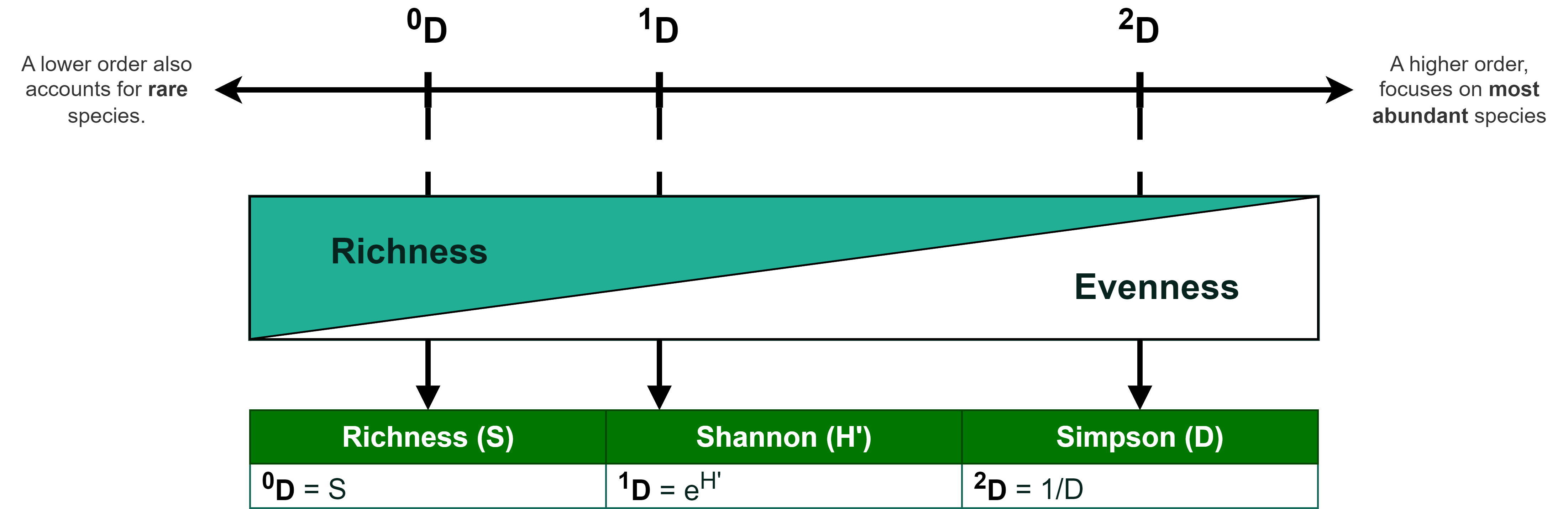
You can choose the diversity order (0, 1, or 2) and this determines how much weight you give to rare species versus dominant ones:
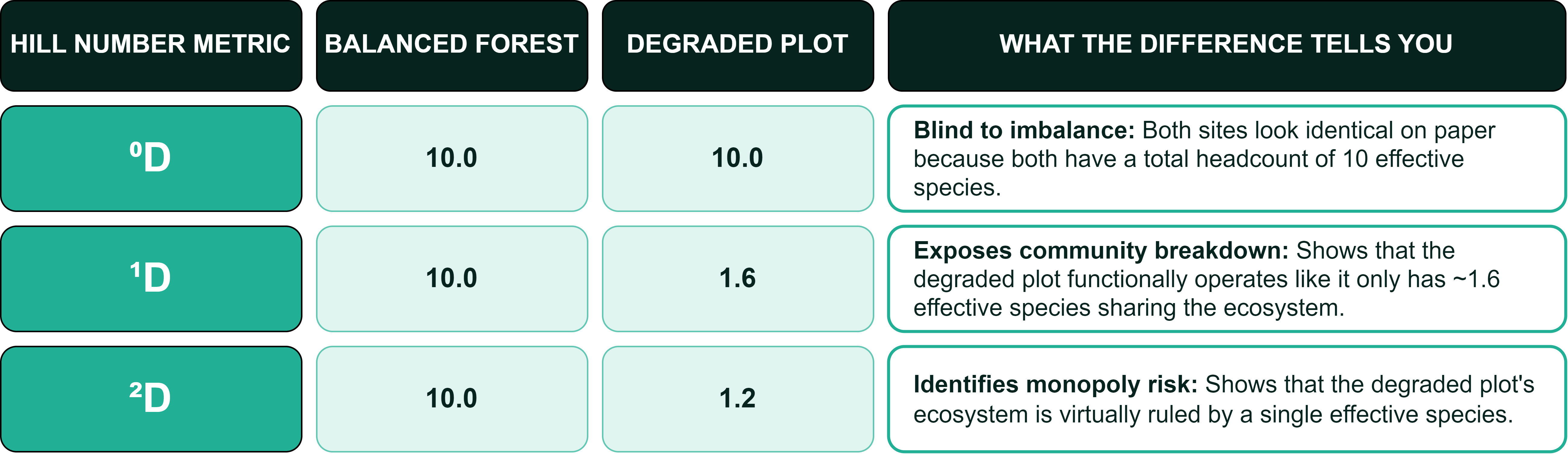
0D: Counts every single species equally, no matter how rare or abundant. (A single sighting of a rare butterfly counts the same as 10,000 ants).
1D: Weighs species proportionally to their abundance. It counts how many typical, common species are in the ecosystem.
2D: Focuses almost entirely on the most abundant wildlife. It tells you how many species are abundant in the ecosystem.
The Hill Numbers answer different business questions:
Example
Using the same example as previously, we have two sites, each containing 1,000 total animals across 10 species:
Balanced forest: Each of the 10 species has 100 individuals (10% each). The populations are evenly balanced, creating a healthy, resilient habitat.
Degraded plot: 910 of the animals belong to one single dominant species (91%), while the remaining 9 species have only 10 individuals each (1% each).
Why should your company use Hill Numbers?
The benefits of Hill Numbers for corporate disclosures are:
Linear year-over-year tracking: Hill Numbers scale linearly. If a land restoration project successfully doubles the diversity of a site, its ¹D score doubles (for example, from 5 to 10 effective species).
Global portfolio comparability: Because ⁰D, ¹D, and ²D are all expressed in the same unit—number of effective species—sustainability managers can plot and compare asset health across global facilities using a single standardized framework.
Ecosystem health diagnostics: Comparing all three values reveals habitat balance at a glance. If ⁰D, ¹D, and ²D stay close in value, the ecosystem is healthy and well-balanced. If you see a steep decline from ⁰D down to ¹D, and ²D (e.g., dropping from 30 to 6 to 2), it flags that the habitat is degraded, revealing that a couple of dominant species are crowding out the rest and the core community (¹D) is collapsing before species disappear from the raw count (⁰D) entirely.
Greenwashing prevention: Reporting all three Hill orders prevents a company from claiming high biodiversity on paper (⁰D = 100 species) when its actual operational footprint is dominated by a handful of invasive weeds (¹D = 3.2 effective species).
Step 3: Calculating your regional footprint
Measuring local site health (alpha diversity) is an important first step, but most corporations operate across multiple facilities, agricultural plots, or supply chains. To understand your company’s total nature impact, you must scale your metrics up using beta diversity. But before we can calculate beta diversity, we need to know gamma diversity.
Continue reading this post for free, courtesy of Lars Wullink.